
Challenge: A global industrial manufacturer's vendor planning team was ordering far more stock than needed per replenishment cycle. For a significant number of SKUs, a single purchase order delivered enough inventory to cover six months or more of actual consumption.
Lot sizes in SAP had been configured based on supplier defaults, historical purchasing habits, or volume discount logic that no longer reflected current demand patterns. Over time, demand shifted, but the lot size parameters stayed static.
The consequences were predictable:
- Working capital was locked in slow-moving inventory sitting on warehouse shelves.
- Warehouse space was consumed by stock that could have been ordered in smaller, more frequent batches.
- Planners had no systematic way to identify which SKUs were overstocked or by how much.
- Supplier minimum order quantities (MOQs) were accepted at face value without data-backed negotiation.
The planning team needed more than a one-time cleanup. They needed a repeatable, data-driven process to continuously right-size lot sizes as demand patterns evolved.
Solution
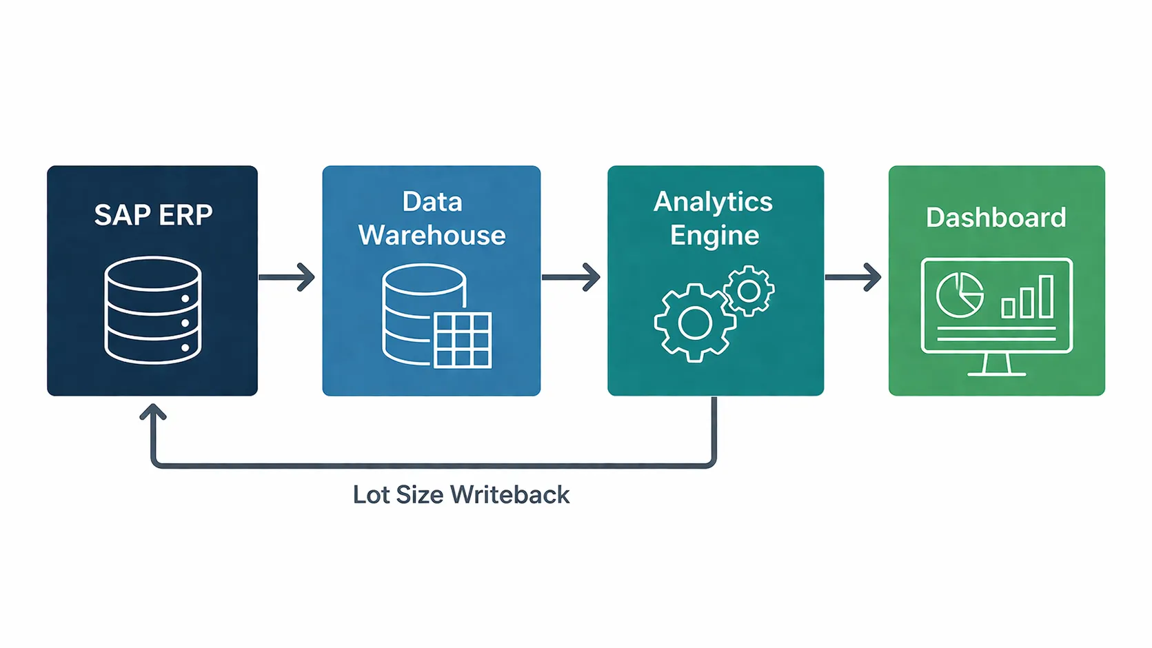
We designed and implemented an analytics workflow that extracted transactional data from SAP, applied demand variability classification and lot size optimization logic, and surfaced actionable recommendations through a Tableau dashboard.
Step 1: Extract and Consolidate Transactional Data
We extracted three critical data sets from SAP into an analytics data warehouse:
- Unit cost per SKU to quantify the capital tied up in each excess lot.
- Current lot size per SKU from SAP's MRP configuration.
- Historical demand by SKU over a rolling 24-month window, used to establish baseline demand and identify variability.
Step 2: Classify SKUs by Demand Stability
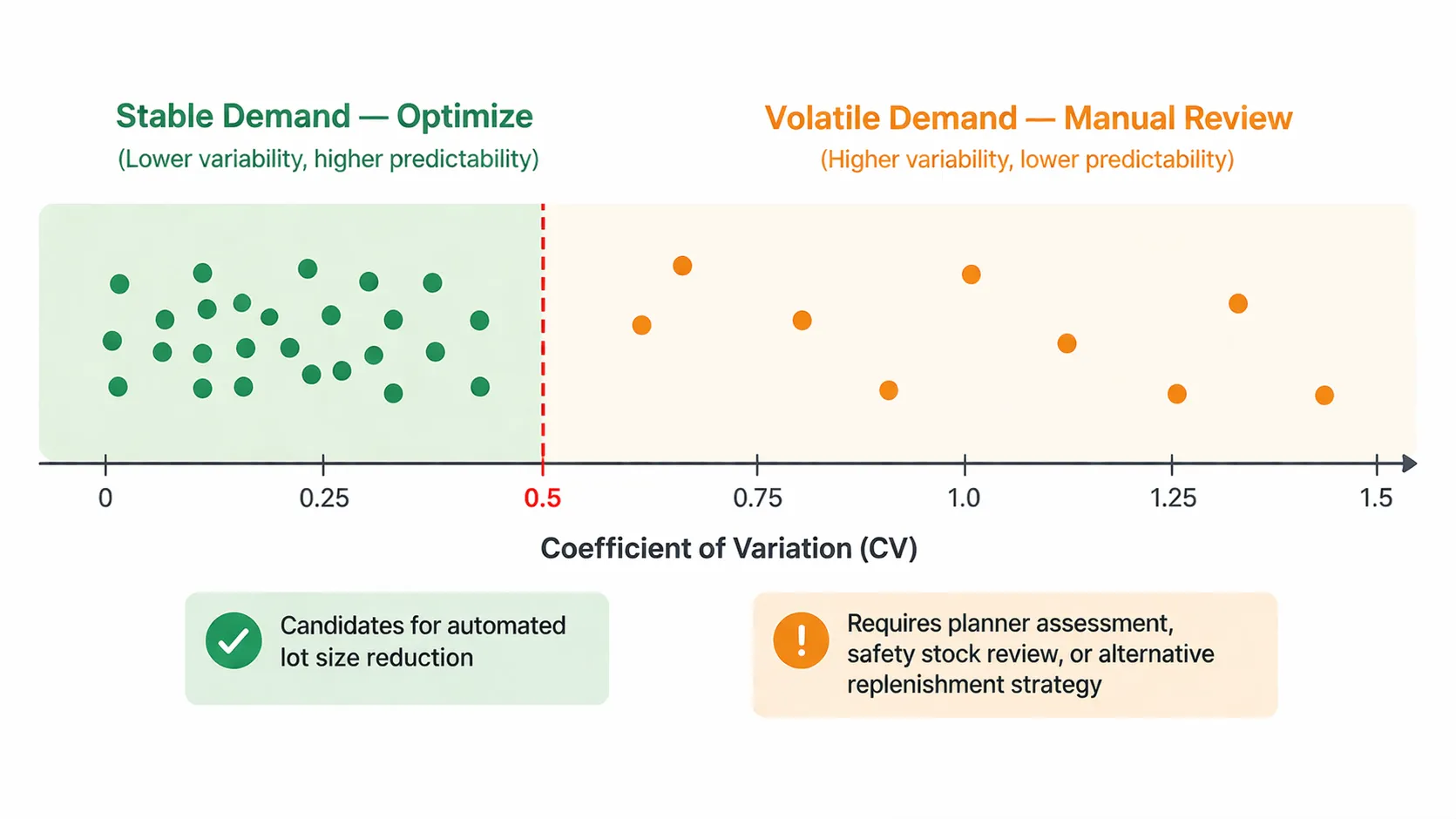
Not every SKU is a candidate for lot size reduction. Items with erratic or highly seasonal demand cannot be safely reduced to smaller, more frequent orders. Doing so risks stockouts during demand spikes.
To separate stable-demand SKUs from volatile ones, we calculated a Coefficient of Variation (CV) for each item:
CV = Standard Deviation of Monthly Demand / Mean Monthly Demand
SKUs with a CV below a defined threshold (typically 0.5 or lower) were classified as having stable, predictable demand, making them suitable for lot size reduction. SKUs above the threshold were flagged for manual review by planners, as they may require safety stock adjustments or a different replenishment strategy entirely (such as make-to-order, consignment, or demand-driven MRP).
Step 3: Calculate Optimal Lot Size
For each qualified SKU, we modeled the optimal lot size by balancing:
- Carrying cost: The cost of holding one unit for one period, including warehouse space, insurance, capital opportunity cost, and obsolescence risk.
- Ordering cost: The fixed cost per purchase order covering administrative processing and inbound logistics.
- Supplier MOQ constraint: The minimum quantity the supplier will accept. If the calculated optimal lot size fell below the supplier's MOQ, the SKU was flagged for MOQ renegotiation with procurement.
- Pack size multiples: Orders must align with physical packaging units (cases, pallets). The optimal lot size was rounded to the nearest feasible pack size multiple.
The model produced a recommended lot size per SKU that minimized total inventory cost while respecting real-world constraints.
Step 4: Quantify the Improvement Opportunity
For every SKU where the recommended lot size was smaller than the current SAP configuration, we calculated:
- Current months of supply per order
- how many months of demand the current lot size covers.
- Recommended months of supply
- the same metric under the optimized lot size.
- Capital freed
- the reduction in average inventory value (unit cost multiplied by the reduction in average units held).
- Shelf space recovered
- estimated pallet positions freed per warehouse.
This produced a ranked opportunity list: the SKUs where lot size reduction would deliver the most capital and space savings, sorted by impact.
Step 5: Operationalize the Recommendations
The analytical output fed two operational workflows:
Direct SAP updates: Where the optimized lot size was above or equal to the existing supplier MOQ, the lot size parameter in SAP was updated directly. The next MRP run would automatically generate purchase orders at the new, smaller quantity.
MOQ renegotiation queue: Where the optimal lot size fell below the supplier's current MOQ, the SKU was routed to the procurement team with a renegotiation brief showing the supplier the demand data, the current overstocking cost, and the proposed new MOQ. Procurement then engaged the supplier to negotiate revised terms, potentially including adjusted pack sizes, more frequent delivery schedules, or revised pricing tiers.
The Dashboard
All outputs were consolidated into a Tableau dashboard published on the organization's Tableau Server, giving the planning team:
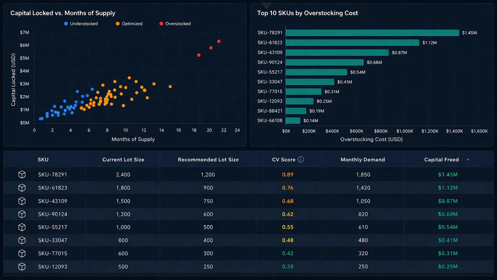
- SKU-level drill-down with current versus recommended lot size, months of supply, CV classification, and capital impact per item.
- Opportunity heatmap showing which SKU and warehouse combinations had the highest overstocking cost.
- Supplier view with aggregated renegotiation opportunities grouped by vendor, enabling procurement to prioritize supplier conversations by total potential savings.
- Trend monitoring that flagged SKUs whose demand patterns shifted from stable to volatile or vice versa, prompting planners to reassess.
The model was refreshed on a defined cycle, ensuring recommendations stayed current as demand evolved and supplier terms changed.
Results
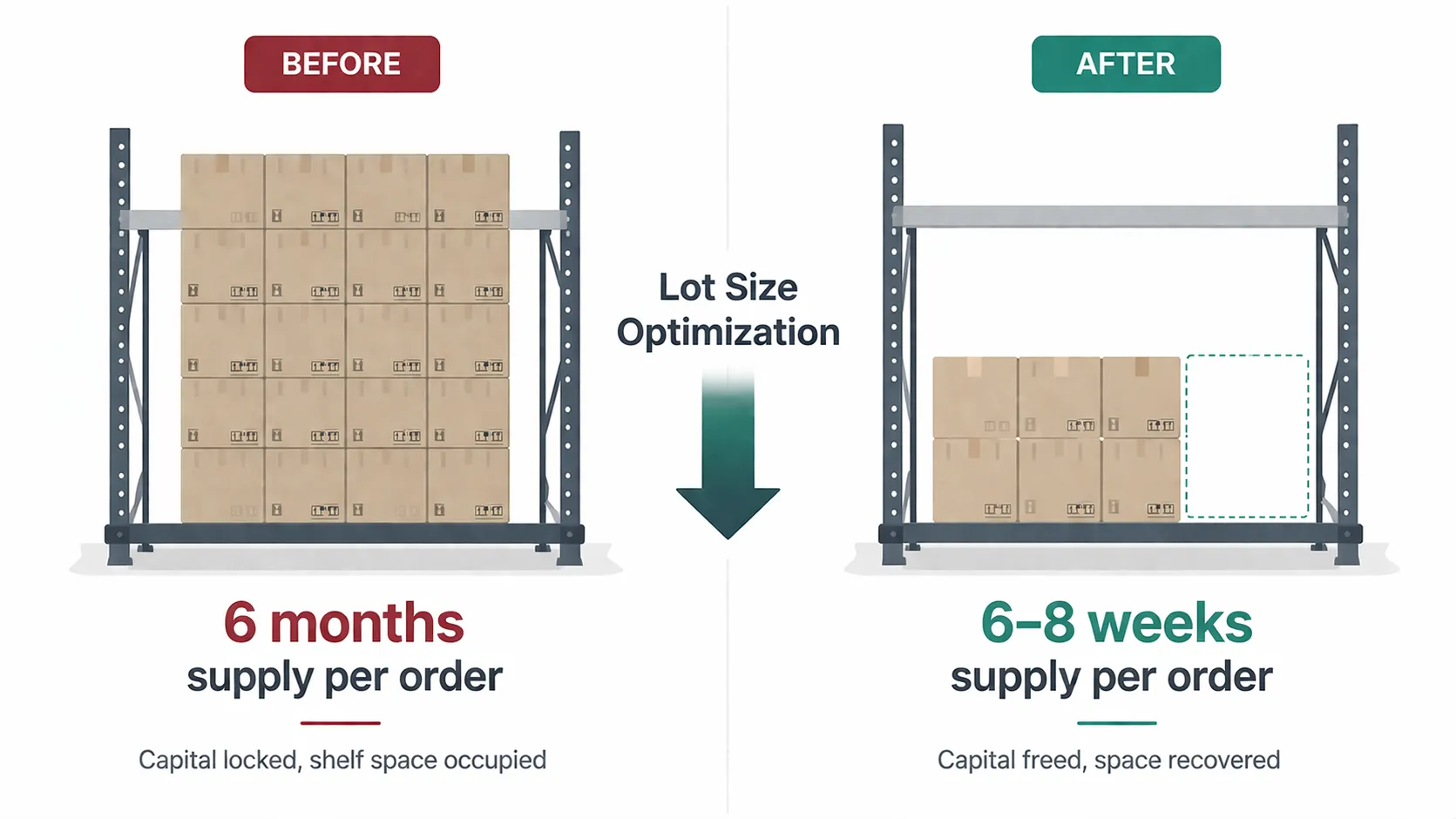
- Identified overstocked SKUs carrying four to six or more months of supply where six to eight weeks would have been sufficient.
- Produced a prioritized list of lot size reductions projected to free significant working capital.
- Generated supplier-specific MOQ renegotiation briefs for procurement, backed by consumption data rather than planner intuition.
- Replaced static Excel-based planning models with a repeatable, automated analytics workflow.
| Scenario | Months of supply per order | Working capital impact |
|---|---|---|
| Before optimization | 4-6+ months | High capital lock-up |
| After optimization | 6-8 weeks | Significantly reduced |
Key Takeaways
Demand variability is the gatekeeper. The Coefficient of Variation filter was essential. Without it, naive lot size reduction on volatile SKUs would have caused stockouts, trading a capital problem for a service level problem.
Lot sizes and MOQs are different levers. Lot size is an internal parameter you control in SAP. MOQ is a supplier-imposed constraint that requires negotiation. Conflating the two leads to recommendations that cannot be implemented. The model respected this boundary clearly.
The data existed, the analysis did not. SAP held all the transactional data needed for this optimization. What was missing was an analytics layer that could consolidate it, apply the logic, and surface actionable recommendations. The gap was not data availability but data activation.
Technologies and Tools
SAP ERP, Azure Synapse Analytics, Alteryx, Tableau Server, Python